By Thisara Priyamal in Machine Learning — 10 Sep 2025

පැරණි Machine Learning Algorithms | Linear Regression, SVM, Decision Trees Sinhala Guide

ආයුබෝවන් යාළුවනේ! අද අපි කතා කරන්න යන්නේ Artificial Intelligence (AI) සහ Machine Learning (ML) ගැන, විශේෂයෙන්ම මේකේ පදනම වෙන Traditional Machine Learning Algorithms ගැන. 'AI' සහ 'Machine Learning' කියන වචන අද හැමතැනම අහන්න ලැබෙනවා නේද? ChatGPT වගේ Large Language Models (LLMs) ගැන කතා කරන මේ වෙලාවේ, සමහර අයට හිතෙන්න පුළුවන් Traditional ML Algorithms දැන් පරණයි කියලා. ඒත් ඒක වැරදියි!

ඇත්තටම, Traditional ML Algorithms තමයි මේ හැමදේකම මුල්ගල. ඒවා තමයි අපිට data patterns තේරුම් ගන්න, predictions කරන්න, decisions ගන්න උදව් කරන්නේ. පොඩි project එකක ඉඳන් ලොකු industrial applications වෙනකල් මේ Algorithms අතිශයින්ම වැදගත්.

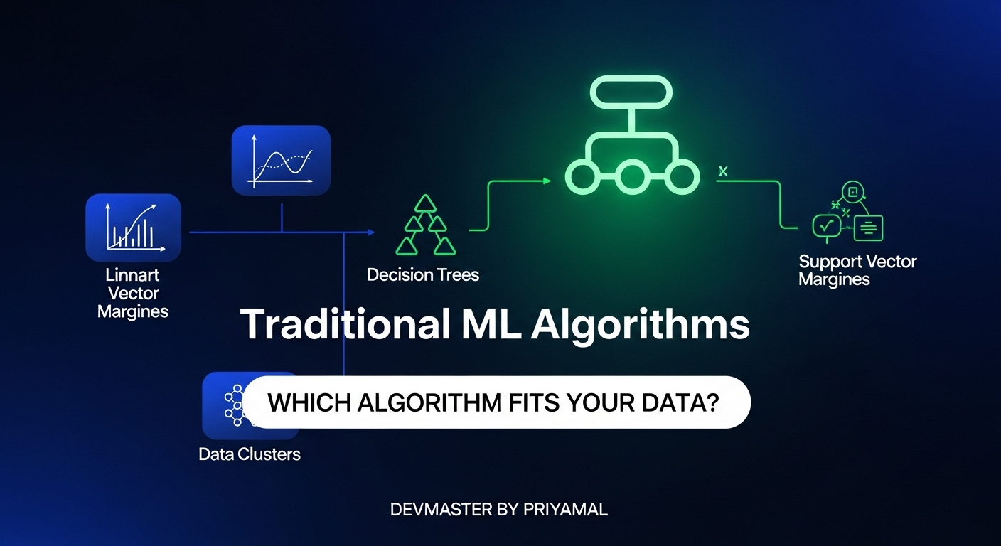
මේ article එකෙන් අපි Linear Regression, Logistic Regression, Decision Trees, Random Forests, සහ Support Vector Machines (SVM) වගේ ප්‍රධාන Traditional ML Algorithms මොනවද, ඒවා කොහොමද වැඩ කරන්නේ, සහ අපිට ඒවා පාවිච්චි කරන්න පුළුවන් කොයි වගේ තැන්වලද කියලා සරලව, පැහැදිලිව කතා කරමු. Python's scikit-learn library එකෙන් අපි මේවා implement කරන හැටිත් බලමු. ඉතින්, කම්මැලි නැතුව, අපි මේ ගමන පටන් ගමු!

1. Regression Algorithms: අනාගතය පුරෝකථනය කරමු - Linear Regression

මුලින්ම අපි බලමු Regression කියන්නේ මොකක්ද කියලා. Regression Algorithms පාවිච්චි කරන්නේ continuous values predict කරන්න. උදාහරණයක් විදියට, ගෙදරක මිලක් (price), කෙනෙක්ගේ වයස (age), නැත්නම් shares වල මිල වගේ දේවල් predict කරන්න. මේවා නිශ්චිත category එකකට වැටෙන්නේ නැති, අඛණ්ඩව වෙනස් වෙන සංඛ්‍යා.

Linear Regression: සරලම පුරෝකථනය

Linear Regression කියන්නේ Regression Algorithms අතරින් සරලම සහ පදනම්ම Algorithm එක. මේකේ ප්‍රධානම අරමුණ තමයි independent variable එක (input) සහ dependent variable එක (output) අතර තියෙන linear relationship එකක් හොයාගන්න එක. සරලව කිව්වොත්, data points අතරින් හොඳටම ගැලපෙන straight line එකක් (regression line) අඳින්න උත්සාහ කරනවා.

ගණිතමය වශයෙන් ගත්තොත්, මේ line එකේ සමීකරණය Y = mX + c කියන form එකෙන් ලියන්න පුළුවන්. මෙතන Y කියන්නේ predict කරන්න ඕන කරන output එක (dependent variable), X කියන්නේ input එක (independent variable), m කියන්නේ line එකේ gradient එක (slope), සහ c කියන්නේ Y-intercept එක. Algorithm එක උත්සාහ කරන්නේ මේ m සහ c කියන values දෙක data points වලට හොඳම විදියට ගැලපෙන විදියට හොයාගන්න එක.

කොහෙද පාවිච්චි කරන්නේ?

ගෙවල් වල මිල predict කරන්න (නිදන කාමර ගාණ, ප්‍රමාණය අනුව).
Stock market එකේ shares වල මිල predict කරන්න.
ව්‍යාපාරික ආදායම් පුරෝකථනය කරන්න.

Python උදාහරණයක්:


import numpy as np
from sklearn.linear_model import LinearRegression
import matplotlib.pyplot as plt

# Sample Data: Home size (sqft) vs. Price (LKR 1000s)
X = np.array([1200, 1400, 1600, 1800, 2000, 2200, 2400]).reshape(-1, 1) # Independent variable
y = np.array([120, 150, 170, 190, 210, 230, 250]) # Dependent variable

# Create a Linear Regression model
model = LinearRegression()

# Train the model
model.fit(X, y)

# Make a prediction
new_home_size = np.array([[2100]])
predicted_price = model.predict(new_home_size)

print(f"Predicted price for a {new_home_size[0][0]} sqft home: LKR {predicted_price[0]:.2f} (1000s)")
print(f"Model coefficients: Slope (m) = {model.coef_[0]:.2f}, Intercept (c) = {model.intercept_:.2f}")

# Plotting the results (optional)
plt.scatter(X, y, color='blue', label='Actual Prices')
plt.plot(X, model.predict(X), color='red', label='Regression Line')
plt.xlabel('Home Size (sqft)')
plt.ylabel('Price (LKR 1000s)')
plt.title('Linear Regression: Home Price Prediction')
plt.legend()
plt.show()

මේ code එකෙන් අපිට පුළුවන් ගෙදරක size එක අනුව මිල predict කරන්න. model.fit(X, y) කියන එකෙන් තමයි algorithm එක data එකෙන් ඉගෙනගෙන m සහ c values හොයාගන්නේ. හරිම සරලයි, නේද?

2. Classification Algorithms: කාණ්ඩවලට වෙන් කරමු - Logistic Regression

Regression Algorithms වගේම තවත් වැදගත් Algorithm වර්ගයක් තමයි Classification Algorithms. මේවා පාවිච්චි කරන්නේ data එකක් යම් නිශ්චිත category එකකට (කාණ්ඩයකට) අයිතිද කියලා predict කරන්න. උදාහරණයක් විදියට, ඊමේල් එකක් spam ද නැද්ද, රෝගියෙක්ට යම් රෝගයක් තියෙනවද නැද්ද, image එකක තියෙන්නේ බළලෙක්ද බල්ලෙක්ද වගේ දේවල් predict කරන්න.

Logistic Regression: නම "Regression" වුණාට වැඩේ "Classification"

Logistic Regression කියන නමේ "Regression" කියන වචනය තිබුණත්, මේක ඇත්තටම classification Algorithm එකක්. මේක binary classification (දෙකකට වෙන් කිරීම) සඳහා බහුලව පාවිච්චි කරනවා.

Linear Regression වගේ මේක straight line එකක් predict කරන්නේ නැහැ. ඒ වෙනුවට, sigmoid function (හෝ logistic function) එකක් පාවිච්චි කරලා, output එක 0 ත් 1 ත් අතර probability (සම්භාවිතාවක්) එකක් විදියට predict කරනවා. 0.5 වගේ threshold (සීමාවක්) එකක් පාවිච්චි කරලා, මේ probability එකට අනුව classification එක කරනවා. උදාහරණයක් විදියට, probability එක 0.5 ට වඩා වැඩිනම් "positive" class එකටත්, අඩුවනම් "negative" class එකටත් classify කරනවා.

කොහෙද පාවිච්චි කරන්නේ?

Spam detection (ස්පෑම් ඊමේල් හඳුනාගැනීම).
Disease prediction (රෝගියෙක්ට රෝගයක් තියෙනවද නැද්ද).
Customer churn prediction (පාරිභෝගිකයන් නැතිවෙයිද කියලා පුරෝකථනය).

Python උදාහරණයක්:


import numpy as np
from sklearn.linear_model import LogisticRegression
from sklearn.model_selection import train_test_split
from sklearn.metrics import accuracy_score

# Sample Data: Study hours vs. Pass/Fail (0 = Fail, 1 = Pass)
X = np.array([0.5, 1.0, 1.5, 2.0, 2.5, 3.0, 3.5, 4.0, 4.5, 5.0, 5.5, 6.0]).reshape(-1, 1)
y = np.array([0, 0, 0, 0, 1, 1, 1, 1, 1, 1, 1, 1])

# Split data into training and testing sets
X_train, X_test, y_train, y_test = train_test_split(X, y, test_size=0.2, random_state=42)

# Create a Logistic Regression model
model = LogisticRegression()

# Train the model
model.fit(X_train, y_train)

# Make predictions on the test set
y_pred = model.predict(X_test)

print(f"Predicted classes for test data: {y_pred}")
print(f"Actual classes for test data:   {y_test}")
print(f"Accuracy: {accuracy_score(y_test, y_pred):.2f}")

# Predict probability for a new student studying 2.7 hours
new_student_hours = np.array([[2.7]])
prediction_prob = model.predict_proba(new_student_hours)
print(f"Probability of passing for 2.7 hours of study: {prediction_prob[0][1]:.2f}") # Probability of class 1 (Pass)

මේ උදාහරණයෙන් පේනවා, LogisticRegression එකෙන් predict_proba කියන method එක පාවිච්චි කරලා probability එක predict කරන හැටි. Accuracy එකත් අපිට බලන්න පුළුවන්.

3. Tree-Based Algorithms: තීරණ ගන්නා ගස් - Decision Trees සහ Random Forests

අපි දැන් බලමු තීරණ ගන්නා ගස් වගේ වැඩ කරන Algorithms ගැන. මේවා බොහොම intuitive (බුද්ධිමය වශයෙන් තේරුම් ගැනීමට පහසු) සහ visual කරන්නත් පහසුයි.

Decision Trees: ගසක් වගේ තීරණ ගැනීම

Decision Tree එකක් කියන්නේ flowchart එකක් වගේ structure එකක්. මේකේ සෑම "node" එකක්ම feature එකක් මත පදනම්ව ප්‍රශ්නයක් අහනවා (උදාහරණයක් විදියට, "Age > 30 ද?"), සහ "branch" එකකින් ඊළඟ "node" එකට යනවා. අන්තිමට "leaf node" එකකින් final decision එක (classification) හෝ value එක (regression) දෙනවා.

වාසි:

තේරුම් ගැනීමට සහ අර්ථකථනය කිරීමට පහසුයි (easy to interpret).
Data preparation එකට ගොඩක් මහන්සි වෙන්න ඕනේ නැහැ (e.g., no need for feature scaling).

අවාසි:

Overfitting වෙන්න පුළුවන් (training data එකට වැඩියෙන් ගැලපීම, අලුත් data වලට හොඳට වැඩ නොකිරීම).
පොඩි data change එකකින් වුණත් tree එක ගොඩක් වෙනස් වෙන්න පුළුවන්.

කොහෙද පාවිච්චි කරන්නේ?

Customer segmenting (පාරිභෝගිකයන් කාණ්ඩවලට වෙන් කිරීම).
Credit risk assessment (ණය අවදානම තක්සේරු කිරීම).

Random Forests: ගස් වනයක බලය

Decision Trees වල overfitting ප්‍රශ්නයට විසඳුමක් විදියට තමයි Random Forests බිහි වුණේ. මේක Ensemble Learning කියන concept එකේ කොටසක්. සරලව කිව්වොත්, Random Forest එකක් කියන්නේ එක එක Decision Trees ගොඩක් (forest එකක්) එකට එකතු කරලා හදපු Algorithm එකක්.

මේක වැඩ කරන්නේ මෙහෙමයි: එකම training data set එකේ random sub-samples අරගෙන, ඒ හැම sub-sample එකකටම වෙනම Decision Tree එකක් train කරනවා. ඒ වගේම, හැම tree එකක්ම train කරනකොට feature selection එකත් random කරනවා. අන්තිමට, හැම tree එකකින්ම ලැබෙන predictions වල "majority vote" (classification) එක හෝ average එක (regression) අරගෙන final prediction එක දෙනවා.

වාසි:

Overfitting අඩු කරනවා (Decision Trees වලට වඩා).
High accuracy එකක් දෙනවා.
Robust (ප්‍රතිරෝධී) වෙනවා noise සහ outliers වලට.

අවාසි:

Decision Trees වලට වඩා තේරුම් ගැනීමට අමාරුයි (black box වගේ).
Training කරන්න වැඩි කාලයක් සහ computational resources අවශ්‍යයි.

Python උදාහරණයක් (Random Forest):


import pandas as pd
from sklearn.ensemble import RandomForestClassifier
from sklearn.model_selection import train_test_split
from sklearn.metrics import accuracy_score

# Sample Data: (Imagine features like 'age', 'income', 'education' for predicting 'loan_approval')
data = {
    'Age': [25, 30, 35, 40, 28, 45, 50, 22, 33, 38],
    'Income': [50000, 60000, 70000, 80000, 55000, 90000, 100000, 45000, 65000, 75000],
    'Education': [12, 16, 14, 18, 12, 16, 18, 10, 14, 16],
    'Loan_Approval': [0, 1, 0, 1, 0, 1, 1, 0, 1, 1] # 0 = No, 1 = Yes
}
df = pd.DataFrame(data)

X = df[['Age', 'Income', 'Education']]
y = df['Loan_Approval']

# Split data
X_train, X_test, y_train, y_test = train_test_split(X, y, test_size=0.3, random_state=42)

# Create a Random Forest Classifier model
model = RandomForestClassifier(n_estimators=100, random_state=42) # n_estimators = number of trees

# Train the model
model.fit(X_train, y_train)

# Make predictions
y_pred = model.predict(X_test)

print(f"Predicted Loan Approval for test data: {y_pred}")
print(f"Actual Loan Approval for test data:   {y_test.values}")
print(f"Accuracy: {accuracy_score(y_test, y_pred):.2f}")

මේ උදාහරණයෙන් පේනවා RandomForestClassifier එක කොහොමද use කරන්නේ කියලා. n_estimators කියන්නේ අපි හදන Decision Trees ගාණ. වැඩි trees ප්‍රමාණයක් accuracy එක වැඩි කරන්න උදව් වෙනවා, නමුත් training time එකත් වැඩි වෙනවා.

4. Support Vector Machines (SVM): හොඳම වෙන් කිරීමේ රේඛාව සොයා ගැනීම

අන්තිමට, අපි කතා කරන්නේ Classification (සහ Regression) දෙකටම පාවිච්චි කරන්න පුළුවන් තවත් බලගතු Algorithm එකක් වන Support Vector Machines (SVM) ගැනයි.

SVM: දත්ත වෙන් කරන "Hyperplane" එක

SVM වල ප්‍රධානම අරමුණ තමයි different classes (කාණ්ඩ) දෙකක් අතර "හොඳම වෙන් කිරීමේ රේඛාව" (optimal hyperplane) හොයාගන්න එක. "Hyperplane" එකක් කියන්නේ data points වෙන් කරන line එකක් (2D නම්), plane එකක් (3D නම්), නැත්නම් multi-dimensional space එකක surface එකක්.

SVM උත්සාහ කරන්නේ මේ hyperplane එක, closest data points (මේවාට "Support Vectors" කියනවා) දෙපැත්තට තියෙන දුර (margin) උපරිම කරන්න. ලොකු margin එකක් තියෙන hyperplane එකක් අලුත්, නොදැකපු data points නිවැරදිව classify කරන්න හොඳටම උදව් වෙනවා.

සමහර වෙලාවට data එක linear විදියට වෙන් කරන්න බැරි වෙන්න පුළුවන්. ඒ වගේ වෙලාවට SVM වල "Kernel Trick" කියන එක පාවිච්චි කරනවා. මේකෙන් කරන්නේ original data එක higher dimensional space එකකට map කරන එක. එතකොට ඒ higher dimensional space එකේදී data එක linear විදියට වෙන් කරන්න පුළුවන් වෙනවා.

කොහෙද පාවිච්චි කරන්නේ?

Image recognition (රූප හඳුනාගැනීම).
Text classification (පෙළ වර්ගීකරණය).
Bioinformatics (ජීව විද්‍යාත්මක දත්ත විශ්ලේෂණය).
Small to medium sized datasets වලට හොඳට වැඩ කරනවා.

Python උදාහරණයක්:


import numpy as np
from sklearn import svm
from sklearn.model_selection import train_test_split
from sklearn.metrics import accuracy_score
import matplotlib.pyplot as plt

# Sample Data: Two features (e.g., 'X1', 'X2') for two classes (0 or 1)
# Class 0: closer to origin
X_class0 = np.random.rand(20, 2) * 2
# Class 1: further from origin
X_class1 = np.random.rand(20, 2) * 2 + 3

X = np.vstack((X_class0, X_class1))
y = np.array([0]*20 + [1]*20)

# Split data
X_train, X_test, y_train, y_test = train_test_split(X, y, test_size=0.3, random_state=42)

# Create an SVM Classifier model
# 'kernel' can be 'linear', 'poly', 'rbf' (radial basis function) etc.
model = svm.SVC(kernel='linear', random_state=42)

# Train the model
model.fit(X_train, y_train)

# Make predictions
y_pred = model.predict(X_test)

print(f"Predicted classes for test data: {y_pred}")
print(f"Actual classes for test data:   {y_test}")
print(f"Accuracy: {accuracy_score(y_test, y_pred):.2f}")

# Note: Plotting decision boundaries is more complex and might clutter a simple tutorial.
# The following commented out section provides an idea, but is not run for brevity.
# Plotting the decision boundary (simplified for 2D)
# plt.scatter(X[:, 0], X[:, 1], c=y, s=30, cmap=plt.cm.Paired)
# # plot the decision function
# ax = plt.gca()
# xlim = ax.get_xlim()
# ylim = ax.get_ylim()
#
# # create grid to evaluate model
# xx = np.linspace(xlim[0], xlim[1], 30)
# yy = np.linspace(ylim[0], ylim[1], 30)
# YY, XX = np.meshgrid(yy, xx)
# xy = np.vstack([XX.ravel(), YY.ravel()]).T
# Z = model.decision_function(xy).reshape(XX.shape)
#
# # plot decision boundary and margins
# ax.contour(XX, YY, Z, colors='k', levels=[-1, 0, 1], alpha=0.5,
#            linestyles=['--', '-', '--'])
# # plot support vectors
# ax.scatter(model.support_vectors_[:, 0], model.support_vectors_[:, 1], s=100,
#            linewidth=1, facecolors='none', edgecolors='k')
# plt.title('SVM Decision Boundary (Linear Kernel)')
# plt.xlabel('Feature 1')
# plt.ylabel('Feature 2')
# plt.show()

svm.SVC (Support Vector Classifier) එකෙන් අපිට පුළුවන් classification කරන්න. kernel='linear' කියන්නේ අපි linear hyperplane එකක් හොයනවා කියන එක. Advanced cases වලට 'rbf' වගේ kernels පාවිච්චි කරන්න පුළුවන්.

අවසානය: මුල්ගල නොදැන ගොඩනැගිලි හදන්න බැහැ!

ඉතින් යාළුවනේ, මේ article එකෙන් අපි Traditional Machine Learning Algorithms කිහිපයක් ගැන දැනගත්තා. Linear Regression වලින් continuous values predict කරන හැටි, Logistic Regression වලින් classifications කරන හැටි, Decision Trees සහ Random Forests වලින් flowchart වගේ තීරණ ගන්න හැටි, සහ SVM වලින් දත්ත වෙන් කරන්න optimal hyperplane එකක් හොයන හැටි ඔයාලට දැන් පැහැදිලියි කියලා හිතනවා.

ChatGPT වගේ LLMs තාක්ෂණයත් එක්ක AI ලෝකය වේගයෙන් දියුණු වුණත්, මේ Algorithms වල වැදගත්කම තවමත් ඒ විදියටම තියෙනවා. මොකද, මේවා තමයි තවමත් ගොඩක් practical applications වලට පදනම වෙන්නේ. ඒවා තේරුම් ගැනීමෙන් තමයි අපිට සංකීර්ණ AI systems වලට යන්න පුළුවන් වෙන්නේ.

ඔයාලට මේ Algorithms ගැන අලුතෙන් මොනවහරි ඉගෙන ගන්න ලැබුණද? ඔයාලගේ project වල මේ Algorithm එකකින් වැඩක් ගත්ත අවස්ථා තියෙනවද? පහළින් comment එකක් දාලා ඔයාලගේ අදහස් අපිත් එක්ක බෙදාගන්න. මතක තියාගන්න, Machine Learning කියන්නේ continuous learning process එකක්. පුහුණු වෙන්න, අත්හදා බලන්න, අලුත් දේවල් ඉගෙන ගන්න!

ඔයාලට ජය!